Wave Divisions
technical Companion Article
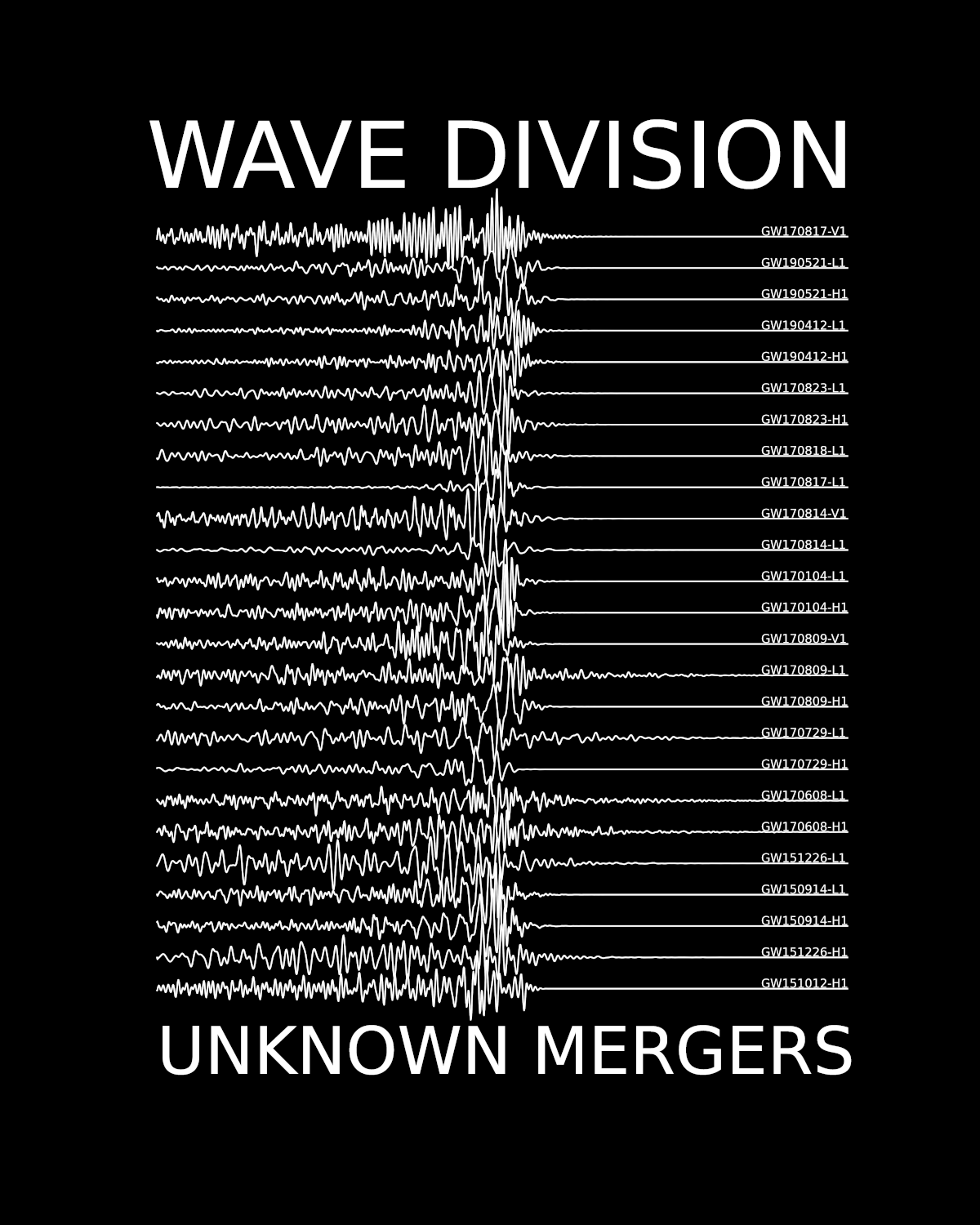
This article is meant to be a complement to Gravitational Wave Division which explains the story behind this image:
These articles are examples of what learning Physics in High School can be like. If you would like to support initiatives like these, order a Wave Divisions T-shirt 👕! $\Longleftarrow$
Math & Physics of Gravitational Waves
A full treatment would require laying a deep foundation in calculus, differential equations, algebra, tensors, modern mechanics and Einstein's relativity. Instead we will give a flavour from those areas using math and concepts available to a curious and motivated high school student.
The most difficult concept to grasp is what these waves are made of. Or the related question, if water goes up & down in a water wave, what goes up and down in a gravitational wave? Before we get there, we will quickly review some math & notation about waves in general.
The Wave Equation
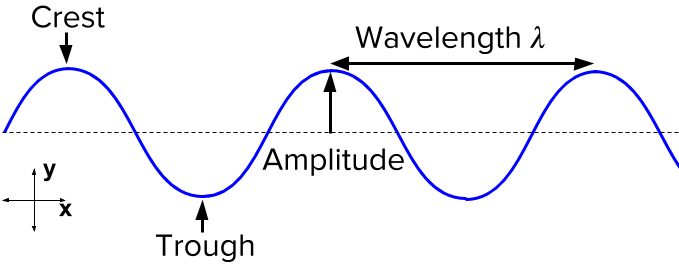
A common equation we learn in high school is $v = \lambda \times f$, where the velocity of the wave $v$ is equal to the wavelength $\lambda$ times the frequency $f$. This assumes the wave is monocromatic (only one wavelength, or only one frequency), and always travels at the same speed. However, that equation says nothing about where the wave is, how high it is, or in which direction it's moving.
For that we need differential equations. If you have learnt how to find a derivative (often written $f'$ or $ \frac{df}{dx} $) you can understand differential equations.
Differential Equations
All Physical laws so far can be written down as equations which combine a variable (time, displacement, electric field, temperature, etc ) and one or more derivatives of that variable. Such an equation is called a differential equation. For example:
$$ F = -kx $$That equation describes the force on a spring. It says, the more you stretch the spring (so, $x$ gets bigger ), the bigger the force $F$ becomes (pointing in the opposite direction of the stretching, thus the minus).
But, as Newton postulated, $F = ma$. But, $a = \frac{\Delta v}{\Delta t}$.
(reminder: $\Delta x$ means, difference between final and initial x,
that's why they are differential equations).
When $\Delta v$ is a tiny difference, we write $\frac{dv}{dt}$. Or said otherwise,
the acceleration is the derivative of the velocity with respect to time.
Now, to save some ink (pixels?) and make equations easier to read, physicists
have a special notation. The dot notation. A dot above a variable means take a time derivative.
So, $\frac{dv}{dt} = \dot{v}$.
So back to our differential equation. The force from a spring is $F = -kx$. but $F = ma = m\dot{v}$. And in fact, $v = \frac{dx}{dt}$. Since the velocity is the derivative of the displacement, we can say: $a = \dot{v} = \ddot{x}$. Putting all this back into our spring equation we have:
$$ \ddot{x} = -\frac{k}{m} x $$In plain English:
Can you find a function $x(t)$ that when you take the derivative twice you get the same function but with a $-\frac{k}{m}$ in front?
Most of Physics can be cast to this process:
- Write down the force
- Put it into Newton's equation
- You will get a riddle about derivatives
- Solve the riddle $\Rightarrow$ get the answer!
Let's solve our riddle! You could try $t^2$, $e^{t^3}$, $3t^k$, and see if it works. However, if you are an expert at derivatives you know a function which comes back to itself with a minus after two derivatives: $$cos(t) \rightarrow -sin(t) \rightarrow -cos(t)$$
With an extra trick, we can make it work:
$$cos( \omega t) \rightarrow -\omega sin(\omega t) \rightarrow -\omega^2 cos(\omega t)$$where we write $\omega$ instead of the cumbersome $\omega = \sqrt{\frac{k}{m}}$.
Now we know that a mass at the end of a spring (without friction) will move a distance away from equilibrium $x(t) = cos(\omega t)$, tracing the shape of a cosine function.
Wave Equations (Water, Ropes, Light)
A similar thing can be done for ropes or water. Pick a bit of mass on the rope, See which forces act on it, plug it into Newton's law... and pray that you can find a function whose derivative does what you need!
Getting the equation is beyond our scope. An overview can be found here and more detail in this PDF.
Imagine a bit of rope which can move up and down a distance $y$,
and the string is layed out along the $x$ axis, like so:
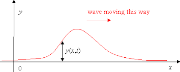
Stating Newton's law for that problem leads to this equation:
$$ \ddot{y} = c^2 \; y_{xx} $$Where $y_{xx}$ is short for, take the derivative of the function $y(x,t)$ with respect to $x$, twice, but ignore the variable $t$, and treat it like a constant. So the riddle this time is:
Can you find a function with two variables ($x$ for position, $t$ for time) $y(x,t)$ so that finding the derivative twice in time gives the same function as finding the derivative twice in position? (Oh, and with a $c^2$ factor).
Amazingly, the equation is super easy so solve. Remember how $cos(t) \rightarrow -sin(t) \rightarrow -cos(t)$?
Well, if you try $y = cos(x-t)$ then:
$$\ddot{y} = - cos(x-t)$$and
$$ y_{xx} = -cos(x-t)$$Woah! I encourage you to see what happens when $t$ increases in that equation. Try it in this simulation.
It sure behaves like a wave, doesn't it? We forgot the $c^2$, but you can check that this solution works:
$$ y = cos(x-ct)$$Go and explore what a big or small $c$ does to our travelling wave. It turns out that $c$ is the speed of the wave.
We can also make the equation more general, in 3D. If the substance or object, can move left-right ($x$), up-down ($y$) and back-forth ($z$), the equation becomes:
$$ \ddot{A} = c^2 \; \left(A_{xx} + A_{yy} + A_{zz}\right) $$Instead of $y(x,t)$, I've used $A(x,y,z,t)$ for the amplitude or displacement of the wave.
It could be the electric field, the height of a wave, or something else that vibrates.
In any case, it's getting a bit boring to write out that many symbols! Physicists are a lazy bunch, so here's another notation trick. You may have noticed that the $A$ is on all terms of the equation. Physicists sometimes like to think of derivatives as operations you apply to something. You could write the wave equation as:
$$ \left[\ddot{\square} - c^2 \; \left(\square_{xx} + \square_{yy} + \square_{zz}\right)\right] A = 0 $$Saying something like: Put the $A$ in each one of those boxes, do all the operations, and you'll get zero. Or, take the time derivative twice, subtract double derivatives in x,y,z with a factor of $c^2$, and you should get zero.
But as I said, physicists are lazy, so they usually shorten the whole wave equation to:
$$ \square \; A = 0 $$That little square which hides 8 derivatives under the hood is called the D'Alambertian. It may not come as a surprise that the equation for gravitational waves is simply:
$$\square \; g_{\mu\nu} = 0$$
But what in the world is $g_{\mu\nu}$?
Einstein's Relativity
Einstein articulated two groundbreaking theories last century: Special Relativity in 2005 and General Relativity in 2015.
Special Relativity
Special relativity describes everything that Newton described, plus what happens when objects travel close to the speed of light. His goal was to marry two requirements:
- Obey the equations of electromagnetism (which describe light, electricity and magnetism)
- That the laws of physics should look the same (be absolute!) for anyone in the universe.
Those seemingly innocent requirements opened Pandora's box. Light is an electric field ($E$) and a magnetic field ($B$). The laws of electromagnetism lead, under certain conditions, to the following equations:
$$ \ddot{E} = \frac{1}{\mu_0 \epsilon_0} E_{xx} $$$$ \ddot{B} = \frac{1}{\mu_0 \epsilon_0} B_{xx} $$You may recognise the familiar wave equation. What is interesting is $\frac{1}{\mu_0 \epsilon_0}$. We said earlier, that a generic wave equation is $$ \ddot{A} = c^2 A_{xx} $$ where $c$ stands for the speed of the wave.
This would mean, that the speed of electromagnetic waves is $$ c = \sqrt{\frac{1}{\mu_0 \epsilon_0} }$$
No biggie? Right? Well, interestingly $\mu_0$ and $\epsilon_0$ have nothing to do with motion. They are constants of nature. $ \sqrt{\frac{1}{\mu_0 \epsilon_0} } $ comes out to be $299\,792 \;\mathrm{km/s}$, which we will approximate to: $300\,000 \;\mathrm{km/s}$ or $3\times10^8 m/s$.
So if Einstein wants these equations to be true, the speed of light must be the same no matter the observer.
If you rush at $250\,000 \;\mathrm{km/s}$ towards a beam of light, it will still appear to move towards you
at $300\,000 \;\mathrm{km/s}$. Equally if you try to catch a beam of light and
run behind it at $298\,000 \;\mathrm{km/s}$, it should still run away from you at $300\,000\;\mathrm{km/s}$. Does that mean light
is moving at $298\,000 + 300\,000$? No. Just $300\,000\;\mathrm{ km/s}$.
Reconciling these seemingly contradictory ideas gave birth to special relativity. Understanding the consequences is beyond our scope, but it introduced a critical question:
How do we measure time, distance and velocity?
The theory of general relativity has some counter-intuitive answers to that question.
A Theory of Metrics
To develop an intuition about general relativity, we need to remind ourselves how we measure distances. Let's start with Pythagoras.
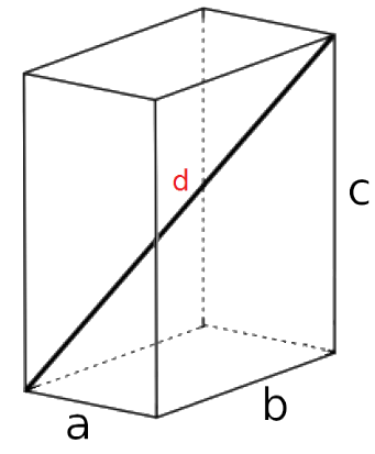
To find a distance $d$ in 3D, we can do: $d^2 = a^2 + b^2 + c^2$.
Or using the usual cartesian variables $(x,y,z)$ and $s$ for displacement, we can rewrite it as: $s^2 = x^2 + y^2 + z^2$.
This way of measuring distances, however, is a convention.
Let's say our axes look like this:
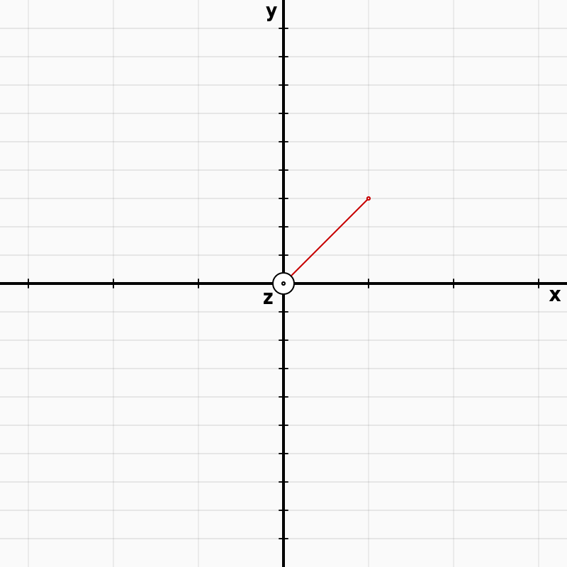
and 1 step in the $x$ direction is as long as 3 steps in the $y$ direction. We can imagine that moving $\sqrt{2}$ meters away from the origin $(0,0,0)$ along the red line, is described by this displacement:
$s^2 = x^2 + \frac{1}{3^2} y^2 + z^2$
So if we move 1 unit in $x$, 3 units in $y$ and zero units in $z$ we travel a distance:
$s = \sqrt{1 + \frac{3^2}{3^2}} = \sqrt{2}$
A formula or rule for finding displacements $s$ is called a metric ). It's kind of a more advanced Pythagorean theorem, useful when steps are not the same size in all directions.
Einstein's General Relativity is all about metrics, and as we will see, the $g_{\mu\nu} $ in our wave equation $\square \; g_{\mu\nu} = 0$ is in fact the metric of spacetime. Inside $g_{\mu\nu} $ are the rules for measuring displacements in spacetime. Now, consider this: how do you measure distances when your coordinate axes misbehave like this?
Surely our metric (the rule to find distances) is now time dependent? Perhaps it will look something like this:
$s^2 = \frac{1}{(2 + sin(t))^2} x^2 + \frac{1}{(2 + 0.3 cos(t))^2} y^2 + z^2$
The time-dependent metric we used is
a little different,
but hopefully it illustrates the point.
Gravitational waves do something similar to this.
They mess with our metric, or our ability to determine distances.
Beware that the analogy only goes so far.
There is no absolute rigid red-line of constant length in the real world.
From Space to Spacetime
Einstein's teacher Minkowski noticed that relativity made a lot more sense if the metric was the following:
$$ s^2 = (ct)^2 - x^2 - y^2 - z^2 $$Where $c$ is the speed of light. In 1908 Minkowski, announced to fellow mathematicians:
[...] space by itself, and time by itself, are doomed to fade away into mere shadows, and only a kind of union of the two will preserve an independent reality
The metric above, in fact, is not just for distances between locations. It finds the distance between events. The word event in Physics has a very specific meaning. It means a point in spacetime. An event has 4 coordinates. Let's write it as $(t, x, y, z)$. If you are standing in your chair at location (2,0,0) at time $t=0$, that is event $(0,2,0,0)$. Even if you don't move, time goes by ... and a second later, you have travelled one second into the future. Your new coordinates are $(1,2,0,0 )$. In the next second you travel 1m in the $x$-direction and land at $(2,3,0,0)$: 3 meters away from $x=0$, and 2 seconds away from $t=0$. How much did you travel in spacetime? Minkowski says the displacement is:
$$ s = \sqrt{(2c)^2 - 1^2}$$You can imagine this as a very, very thin pizza slice. In the time direction we travelled $2\mathrm{s}\times 300\,000 \mathrm{km/s} = 600\,000 \mathrm{km}$ and in the x-direction we travelled $0.001\mathrm{km}$. Only light can create non-thin pizzas slices. In a second, it can move $300\,000 \mathrm{km}$ in the time direction and $300\,000 \mathrm{km}$ in the $x$-direction, making a nice isosceles triangle.
Notation for Metrics:
Before we move on to General relativity we are going to change our notation for metrics. In calculus, instead of writing "a tiny distance $s$" we just use the symbol $ds$. This is a single symbol, even if it has two letters in it. Therefore, Pythagoras for a tiny tiny distance $ds$ can be re-written as:
$$ ds^2 = dx^2 + dy^2 + dz^2 $$$ds$ is sometimes called a line element, or a little part of a line. A curve is made of little line elements one after another. Our line element can also be written in the language of matrices. If you don't know how to multiply matrices and vectors, here's a quick introduction, and a Kahn Academy unit. You will find that.
$$ ds^2
= \left(\begin{matrix} dx & dy & dz \end{matrix} \right)
\left(\begin{matrix} 1 & 0 & 0 \\ 0 & 1 & 0 \\ 0 & 0 & 1 \end{matrix} \right)
\left(\begin{matrix} dx \\ dy \\ dz \end{matrix} \right)
$$
This may seem pretty complicated. Why multiply 2 vectors and a matrix, instead of simply writing $dx^2 + dy^2 + dz^2 $? The idea is to help us see more clearly the
factors in front of the $dx^2, dy^2, dz^2$. The matrix in the middle is what we are interested in. In flat spacetime, this becomes
To make our life easier we take c=1 (speed of light = 1). To do this all we have to do is make up some new units. For example I hearby invent the Mitur. 1 Mitur = 300,000,000 meters. So c = 1 Mitur/s. From now on, we'll use those units.
Next, we'll use the same symbols for all coordinates. So instead of writing $(cdt, dx, dy, dz)$ we will use $(x_0, x_1, x_2, x_3)$. To save pixels and typing, we shorten it like so:
$$ x^\alpha = (x_0, x_1, x_2, x_3)$$where $\alpha$ is assumed to run from $0 \rightarrow 3$. The vector can be transposed like so:
$$ x_\alpha = \left( \begin{matrix} x_0\\ x_1 \\ x_2 \\ x_3 \end{matrix} \right)$$Notice the subtle but important difference between $x^\alpha$ and $x_\alpha$. The first one is a row, and the second a column. At last, we are ready to define the metric in General Relativity. Measuring tiny displacements in spacetime is done like so:
$$ ds^2 = dx^\alpha \left(\begin{matrix} g_{00} & g_{01} & g_{02} & g_{03} \\ g_{10} & g_{11} & g_{12} & g_{13} \\ g_{20} & g_{21} & g_{22} & g_{23} \\ g_{30} & g_{31} & g_{32} & g_{33} \end{matrix} \right) dx_\alpha $$The matrix in the middle is called the metric and tells us how to measure spacetime. It is usually shortened as $$g_{\mu\nu}$$ Where $\mu$ and $\nu$ can have values between $0$ and $3$. So, $g_{\mu\nu}$ is short for a matrix with 16 elements called $g_{00}, g_{01}, ..., g_{33}$. Unlike the simple pythagorean distance which has all zeros outside the diagonal of the matrix, this distance contains terms like $g_{20} dx_2 dx_0$, or $g_{20} dydt$. So, in general, if you move a little along $y$ and then along $t$ you get something different than if you move diagonally along $dydt$.
Surprisingly, no matter where an observer is, or whether or not they are moving with constant velocity $ds^2$ is always the same number relativity. The $g_{\mu\nu}$ elements in the matrix will grow and shrink as needed to make the spacetime-displacement a conserved quantity under such changes of coordinates. Note that changing coordinates changes the metric. For example, in flat spacetime, using cartesian coordinates the metric is:
$$
g_{\mu\nu} =
\left(\begin{matrix} 1 & 0 & 0 & 0 \\ 0 & -1 & 0 & 0 \\ 0 & 0 & -1 & 0 \\ 0 & 0 & 0 & -1 \end{matrix} \right)
$$
but we could just as well use spherical coordinates and have:
$$
g_{\mu\nu} =
\left(\begin{matrix} -1 & 0 & 0 & 0 \\ 0 & 1 & 0 & 0 \\ 0 & 0 & r^2 & 0 \\ 0 & 0 & 0 & r^2sin^2\phi \end{matrix} \right)
$$
Where our coordinates are now $(t, r, \phi, \theta)$ and our line element becomes: \begin{equation*} \displaystyle{ds^2=-dt^2 + dr^2+r^2d\phi ^2+r^2sin^2\phi d\theta ^2} \end{equation*}
and the angles are defined as follows:
![The spherical coordinate system, where θ ∈ [0, π ] is the polar angle, ϕ ∈ [0, 2π ) is the azimuthal angle and r is the distance from the origin: (π/2 − θ ) is the conventional angle of latitude, so that the North Pole corresponds to θ = 0, the South Pole to θ = π , and the Equator to θ = π/2.](https://www.researchgate.net/publication/316068127/figure/fig3/AS:669044097179674@1536523951532/The-spherical-coordinate-system-where-th-0-p-is-the-polar-angle-ph-0-2p-is.png)
Einstein's Toolbox
This opens up an entire field of mathematics which we will not explore, but we want you to have an intuition about the tools in Einstein's box:
- The equations of Physics do not separate $t$ and $(x,y,z)$, instead they talk about spacetime coordinates $x^\alpha = (x^0, x^1, x^2, x^3)$.
- Finding distances is not done using Pythagoras. Instead, some directions in space may shrink or stretch. How much they do in each direction is contained inside the numbers of matrix $g_{\mu\nu}$.
- The metric $g_{\mu\nu}$ helps us find $ds$, how far you travel if you move in a certain space-time direction. In general $g_{\mu\nu}$ can change with time and location.
Einstein's GR Equation
Armed with the tools from the past section, we can ask ourselves: What is the equivalent of Newton's law in Einstein's General Relativity? How do we know the trajectory that a particle will follow? The answer is both surprisingly complex and simple.
If we ignore the expansion of the universe for a second, Einstein discovered the following equation after a decade of laboring:
$$ G_{\mu\nu} = \frac{8\pi G}{c^4} T_{\mu\nu} $$This describes most of general relativity.
The left side is about the shape of space. The curvature of space and how to measure distances (the metric) are given by: $$G_{\mu\nu} = R_{\mu\nu} - \frac{1}{2}R g_{\mu\nu}$$
$R_{\mu\nu}$, called the Ricci tensor, and $R$, called Ricci curvature hide a lot of complexities. They tells us about the curvature of spacetime. Try to imagine the wobbly axes in the gif animation above. Now, extend it to 3 dimensions, and take derivatives everywhere, over time, to identify slopes, gradients and shapes in spacetime. All that hides inside $R_{\mu\nu}$.
The $g$ tells us how to measure distances along $dx$, along $dt$, but also along weird
combinations like along $dx\; dz$ or $dt\; dy$.
The right side of the equation, $\frac{8\pi G}{c^4} T_{\mu\nu}$, is about what is inside of that space (energy, mass, etc). $\frac{8\pi G}{c^4}$ is a tiny constant ($2 \times 10^{-43} N^{-1}$) which multiplies $T_{\mu\nu}$. So $T$ needs to be pretty big to matter! Inside this matrix $T_{\mu\nu}$ are the energies and masses which bend spacetime:

All those $\mu \nu$ indexes let us know where we are on the matrix. For example, $\mu =0, \nu=1$ stands for time and x-direction. Thus, Einstein's equation is not one equation, but 16 of them, one for each element in the matrix! Taking $\mu =0, \nu=1$ one of those equations is:
$$ R_{01} - \frac{1}{2}R g_{01} = \frac{8\pi G}{c^4} T_{01} $$Where derivatives are hiding inside of $R_{01}$ and $T_{01}$. If we wrote out all the multiplications and indexes it would give 10 coupled, non-linear, second-order, hyperbolic-elliptic partial differential equations for the metric components $g_{\mu\nu}$.
If that sounds scary, it is. Nobody knows how to solve them. People have only managed to find solutions by setting most things to zero, approximating and assuming symmetry. For example, nobody knows how to find the exact solution for the moon orbiting the earth!
From GR to Waves in the Metric
If you made it this far. Congratulations! You are ready to have a glimpse at the tools used by physicists to predict gravitational waves. Let me remind you that our goal is not to show all the steps and justify all the details. Instead we want to get a feel for the type of math and physics behind gravitational waves.
It all starts with a simplification. Take Einstein's GR equation,
$$ G_{\mu\nu} = \frac{8\pi G}{c^4} T_{\mu\nu} $$And assume space is totally empty. No mass, no light, no electric or magnetic fields. Just empty. That means $T_{\mu\nu} = 0 $, or
$$ G_{\mu\nu} = 0 $$also written in more detail as: $$ \tag{1} R_{\mu\nu} - \frac{1}{2}R g_{\mu\nu} = 0$$
Easy peasy then! Well. Not so fast. Let's look inside $R_{\mu\nu}$. Before we look inside, lets remind ourselves that $\sum_{i} A_i$ will be short for $\sum_{i=0}^{3} A_i = A_0 + A_1 + A_2 + A_3$ or add up along index $i$ from zero to three. Also, that $\partial_{x_0}$ or $\frac{\partial}{\partial x_0}$ means take the derivative with respect to variable $x_0$. It turns out that:
\begin{equation} \tag{2} R_{\mu\nu} = \sum_{i} \left( \frac{\partial}{\partial x_i} \Gamma_{\mu\nu}^{x_i} - \frac{\partial}{\partial \nu} \Gamma_{\mu x_i}^{x_i} - \sum_{j} \left[ \Gamma_{\mu\nu}^{j} \Gamma_{j x_i}^{x_i} - \Gamma_{\mu x_i}^{j} \Gamma_{j \nu}^{x_i} \right] \right) \end{equation}If you are not yet confused. Remember that everything with two indexes is a matrix ... and inside those matrices are derivatives of some newly introduced variable $\Gamma$. But it gets worse! $\Gamma$ has its own sums with derivatives of the metric! Consider the first $\Gamma_{\mu\nu}^{x_i}$ in the equation above. Inside of it we have:
$$ \tag{3} \Gamma_{\mu\nu}^{x_i} = \frac{1}{2} \sum_{k} g^{x_i k} \left( \frac{\partial}{\partial \nu} g_{\mu k} + \frac{\partial}{\partial \mu} g_{\nu k} - \frac{\partial}{\partial k} g_{\mu \nu} \right) $$Each one of those $\Gamma$ letters in $R_{\mu\nu}$ is a similar animal. Remember what a differential equation is. An easy one was $ \ddot{x} = -\frac{k}{m} x $, or find a function which becomes itself after two time derivatives. General relativity is all about finding 16 functions $g_{\mu \nu}(x,y,z,t)$ that will obey the scary equations above. You can imagine that $R_{\mu\nu}$ contains ideas of the type:
- The space is curved here, and the reference frame is stretched here but not here.
- If you take derivatives around this line, do they grow, change oscillate?
- All that happens in all coordinates (including time which can stretch and elapse slower).
Solving this in general is too hard, so our next simplification is to admit that in most places in the universe, spacetime is mostly flat. Only black holes or neutron stars can stretch things significantly. So when gravitational waves travel, they will create tiny ripples on a mostly flat spacetime. A line element will be almost equal to:
$$ ds^2 = -dt^2 + dx^2 + dy^2 + dz^2 $$but not quite. Our metric will be close to the flat one, but we introduce a matrix $h_{\mu\nu}$ with very very small values for each of the $h$ inside. The metric will then look like this:
$$ g_{\mu\nu} = \left(\begin{matrix} 1 & 0 & 0 & 0 \\ 0 & -1 & 0 & 0 \\ 0 & 0 & -1 & 0 \\ 0 & 0 & 0 & -1 \end{matrix} \right) + \left(\begin{matrix} h_{00} & h_{01} & h_{02} & h_{03} \\ h_{10} & h_{11} & h_{12} & h_{13} \\ h_{20} & h_{21} & h_{22} & h_{23} \\ h_{30} & h_{31} & h_{32} & h_{33} \end{matrix} \right) $$To save space, this is often simplified as:
$$ g_{\mu\nu} = \eta_{\mu\nu} + h_{\mu\nu} $$Where $\eta_{\mu\nu}$ is the easy metric in flat space. Inserting this back into equation (1) which contains equation (2) which itself contains equation (3) is an adventure of its own. But since all terms in $h$ are small, calculations ignore any terms with $h^2$ or $h^3$ ... which will be too tiny to show up in any experiment. After an arduous subsitution exercise, variable renaming and changes of variable ... the following emerges: assuming a tiny change ($h$) to the flat metric $\eta$ of spacetime, equation (1) simplifies to: $$\square h_{\mu\nu}^{\dagger} = 0$$
Which is a wave equation! At last. We have waves in the metric! Einstein himself found that solution to the equations, but it took a century to measure them.
Closing Remarks
As you can imagine we have omitted many steps, concepts and ideas. Each jump where we lose the reader is a field of its own. We hope that at least one reader's curiosity will be peaked and she or he will go on to revolutionize Physics.
If you would like to support educational projects like these, order a Wave Divisions T-shirt 👕! $\Longleftarrow$
Further Reading
Waves
General Relativity - Intuition
- General Relativity for Laypeople - a primer
- The Equivalence principle & the deflection of light
- time dilation in GR
- What is space - nautil.us
General Relativity - full on!
- A no nonsense introduction to General Relativity - Sean Caroll
- Lecture notes on General Relativity - Sean Caroll
- Introduction to general relativity - H. Blöte
- Metric, curved space & General relavivity - Syksy Räsänen
- Edbert's GR 1
Gravitational Waves - Intuition
- Studying the universe with gravitational waves
- Relativistic Astrophysics lecture - Wheeler (intuition + partial derivation)
- Piled Higher and Deeper Explanation
Abridged derivations of gravitational waves
- https://www.quora.com/What-is-the-wave-equation-of-gravitational-waves
- https://www.pnas.org/content/pnas/113/42/11662.full.pdf
Detailed derivation of gravitational waves
- https://arxiv.org/pdf/1005.4735.pdf
- https://www.tat.physik.uni-tuebingen.de/~kokkotas/Teaching/NS.BH.GW_files/GW_Physics.pdf
- https://www.ams.org/publications/journals/notices/201707/rnoti-p684.pdf
- Calibrating and Improving the Sensitivity of the LIGO Detectors, Kissel
 Created in