8 Oct 2020

A stablecoin exchange¶

Curve is an exchange designed for stablecoins and bitcoin tokens on Ethereum. The key aspect of Curve is its market-making algorithm, which can provide 100-1000 times higher market depth than Uniswap or Balancer for the same total value locked.

Curve's Goals¶

The main goal is to let users and other decentralised protocols exchange stablecoins (DAI to USDC for example) through it with low fees and low slippage.

Structure of this Article:¶

You can think of CURVE as a specialized version of the Uniswap exchange. To understand CURVE, we will examine how the Uniswap market making algorithm works. In this article we identify its weaknesses and limitations. Using the lessons learnt we generalize to pools with several coins and finally what problem CURVE is solving and how.

Uniswap's AMM algorithm
Curve's AMM algorithm

1. Uniswap's AMM algo¶

In its simplest form, Uniswap's pricing and trading algorithm can be summarised as:

$$ x \cdot y = k $$

Which means, that if the pool has x tokens of asset X and y tokens of asset Y, then the pool will update its assets such that before and after the trade, $x \cdot y = k$.

$k$ is called the invariant (invariant = thing that stays the same). For example:

there are 1000 X tokens and 5000 Y tokens $x \cdot y = 5 \times 10^6$

Somebody wants to buy Y tokens. To do so, they deposit 200 X tokens into the pool. After the 0.3% fee, 199.4 X tokens are added. The pool now has:

1199.4 X tokens.

The invariant $k = 5 \times 10^6$ has to stay the same, so: $1199.4 \cdot y = 5 \times 10^6$ must be true. We can therefore solve the equation and get: $y = 4168.75$ tokens. In other words, to preserve the invariant $k$, $y = 5000$ needs to go down to $y = 4169.75$. The difference $5000-4168.75 = 831.25$ is how many Y tokens the trader will receive.

uniswap 1/x

Price Setting¶

You may have noticed that the price was automatically set. The trader deposited 200 X and got 831.25 Y, so the price is: $$\mathcal{P} = \frac{831.25}{200} \;\; Y/X$$

or $$\mathcal{P} = 4.16 \;\; Y/X $$

Price Updating¶

What is the price if a new trader wants to trade another 200 X tokens for Y tokens? Well, let's apply $x \cdot y = k$ again to find out:

The new state of the pool after the deposit is:

(1199.4 + 199.4) X tokens

4168.75 Y tokens

So this time we need to solve $1398.8 \cdot y = 5 \times 10^6$. the solution is $y = 3574.4$, so the second trader will get (what_is_currently_in_the_Y_side - what_should_be_in_the_Y_side) $= 4168.75-3574 = 594.75 $. As you see, the second trader got less for her money. The price was:

$$\mathcal{P} = 2.97 \;\; Y/X $$

Y got much more expensive after the first trade! In some ways this makes sense. In the first operation, somebody tried to buy $\frac{831}{5000} ~ 17\% $ of all Y tokens from the pool. In the face of such high demand, the pool auto-adjusted the price accordingly.

Price Equation & geometrical interpretation¶

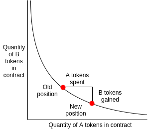
Notice that the price was calculated as $\mathcal{P} = \frac{\Delta y}{\Delta x}$. In other words,

$$\mathcal{P} = \frac{\textrm{how much was taken out}}{\textrm{how much was deposited}}$$

If we think of the $xy=k$ as a curve, the curve $y = \frac{k}{x}$, then $\mathcal{P} = \frac{\Delta y}{\Delta x}$ is its gradient or, in the limit of small trades, the derivative:

$$\mathcal{P} = \frac{d y}{d x}$$

This idea will come back later several times.

In the graph above, as trading occurs, and we have less Y in the pool, but more X:

if the tangent is shalow, you get less Y for your X (Y more expensive, low number)
if the tangent is steep, you get more Y for your X (Y is cheaper)

Slippage¶

In a standard exchange, the order-book: Order Book

Allows us to read how the price will change (slippage) as we buy more and more of a token (travel up the curve). This depends on the details of the price and volume set by each trader. In the AMM, the $x \cdot y=k$ equation and depth of the pool determines this slippage.

For example, What if a single buyer had deposited 400 X tokens, instead of two subsequent buyers? This would have gotten us a price $\mathcal{P} = 3.56\;\; Y/X$, an average between the prices of the first and second buyer.

Depth & Slippage¶

To find the slippage, we compare the price ($\mathcal{P}$) before and after the trade. Since the price is the derivative, we can say that if we exchange $\delta$ tokens of X the slippage is:

$$ \frac{\left. \frac{dy}{dx}\right|_{x} - \left. \frac{dy}{dx}\right|_{x+\delta}}{\left. \frac{dy}{dx}\right|_{x}} $$

Since $\frac{dy}{dx} = \frac{-k}{x^2}$ for $y = \frac{k}{x}$, After substitution and rearrangement the slippage $\mathcal{S}$ is:

$$ \mathcal{S} = 1 - \left(\frac{x}{x+\delta}\right)^2 $$

To interpret this formula we can look at two obvious limits:

If we buy a small amount of X, then $\delta << x$, so $\frac{x}{x+\delta}$ approaches $1$, and slippage tends to zero.
For a deep pool, $x \rightarrow \infty$, so slippage also approaches 0.

Therefore, to avoid price swings, deep liquidity is required. If we rework the numbers with:

X as 1M tokens

Y has 5M tokens

$k = 5 \times 10^{12}$

and deposit X tokens a few times, you can see that the price will be very stable:

Trade Nr	# of X exchanged	Price (Y/X)
1	10	4.9849
2	10	4.9848
3	10	4.9847

or even:

Trade Nr	# of X exchanged	Price (Y/X)
1	10,000	4.9
2	10,000	4.8
3	10,000	4.7

The initial price, of course is given by the initial $\frac{y}{x} = 5$ ratio (gradient at x = 1M).

Arbitrage & Equilibrium¶

In an efficient market, however, traders will spot these arbitrage opportunities. Just like the price of Y was increasing, the price of X (denominated in Y) will be decreasing. Arbitrageurs will buy Y elsewhere and try to sell it in this pool (or buy X in the pool, and sell it, for example in a high volume centralized exchange). For a token with high liquidity elsewhere the short term dynamics may look more like so:

For a Uniswap simulation with real data, see this 30s video

Draining the Pool¶

Even with little depth, if the tokens are traded elsewhere with some degree of liquidity, draining the pool is expensive. Let's consider a pool with:

100 ETH tokens

35,000 USDC tokens

We want to buy all USDCs in the pool. To do so, we will buy USDC by exchanging 100 ETH at a time. The first transaction gets us 17473 USDC, which means the average price of this first transaction is 174 USDC/ETH. The balance in the pool has now moved to 200ETH tokens and 17527USDC, so the price is now 17527/200 ~ 87 USDC/ETH.As we drain the pool we can see how the total money spent (assuming the 100 ETH were bought elsewhere at 350 USD/ETH) rises up the $x \cdot y = k$ curve.

This demonstrates that it is hard to run out of tokens, as long as the tokens don't lose value in the markets.

FEES DISCLAIMER: To make our calculations easier, we have ignored what happens to the fees. The 0.3% is usually returned to the pool. This means that the invariant is not actually invariant and grows over time (by a 0.3% of the deposited pair with every trade, after the trade)

2. Curve's AMM algorithm¶

At a high level, Curve's AMM is a middle ground between Uniswap's product invariant protocol and a linear invariant protocol. Mathematically, it combines:

$$ x \cdot y = k \; \mathrm{and} \; x + y = C$$

curve

This can be generalized to any number of tokens. For 3 tokens, we have:

$$ x \cdot y \cdot z= k \; \mathrm{and} \; x + y + z = C$$

And for $N$ tokens in any proportion,

$$ \prod_{i=1}^{N} x_i^{\omega_i} = k \; \mathrm{and} \; \sum_{i=1}^{N} \alpha_i x_i = C$$

Zero Slippage AMM?¶

Let's imagine an AMM with zero slippage. This means that the derivative $\frac{dy}{dx}$ of the curve is always the same for all $x$. In other words, it is a linear function, or $y \propto x$.

Coming back to our previous example of:

there are 1000 X tokens and 5000 Y tokens

Transactions could obey the equation: $$5000 x + 1000 y = 10000 $$ or $$ y = -5x + 10$$

Here, the price would be $\left|\frac{dy}{dx}\right| = 5$, no matter how much X or Y there is in the pool.

Our curve would look like this:

Where the red dot shows was happens as we add X and widthdraw Y. The invariant is now the total value in the pool. Since X has a value 5 times larger than Y, then 10,000 Y tokens has the same value as 2000 X tokens.

No slippage is no good!¶

Unfortunately, these linear-invariants (generally $\sum_{i=1}^{N} \alpha_i x_i = C$) are not good at keeping the pool balanced. The total value may remain constant, but you can end up running out of tokens. As we saw, the $x \cdot y=k$ pool self-regulated, making it more and more expensive to bring it out of balance.

CURVE tries to achieve a compromise between Low slippage and Stable & Balanced pool.

The curve compromise¶

Curve is a pool for stablecoins. As stablecoins tend to be, well, stable in price, you can take a bit more risk assuming low volatility compared with a random volatile token on Uniswap. However you don’t want the pool sliding up or down a $x+y=k$ curve leading to a single stablecoin. At some point, Curve needs to make it expensive to continue swapping (Like a $xy=k$ exchange does).

To recap, the token price should remain stable and the pool should remain balanced. To do so, Curve creates a linear invariant around the \$1 value, which becomes a product invariant as the tokens depart away from \$1. As shown in the whitepaper, the curve is a combination of $xy=k$ and $x+y=C$

curve comparison

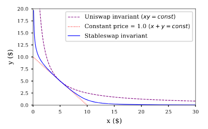
We thus combine the sum invariant of stablecoins: $\sum x_i = D$ with the product invariant $\prod x_i = \left(\frac{D}{n}\right)^n$, where $D$ is the total number of coins when they have an equal price.

For example, the Curve DAI-USDC pool could be governed by:

$$\mathrm{DAI} + \mathrm{USDC} = 30M$$

and $$\mathrm{DAI} \cdot \mathrm{USDC} = \left(\frac{30M}{2}\right)^2$$

Note that the first equation is a sum without coefficients because both start as stablecoins (with an average value of $1$). A first idea could be to add up those two equations. Adding the two equations leads to:

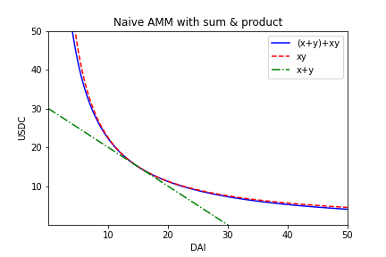
$$\left(\mathrm{DAI} + \mathrm{USDC}\right) + \left(\mathrm{DAI} \cdot \mathrm{USDC} \right) = 30M + \left(\frac{30M}{2}\right)^2$$

What does this curve look like? Rearranging $x+y +x\cdot y = 30 + \frac{30^2}{2^2}$, we obtain this plot:

As you can see, not much has improved in terms of low slippage. Our naive Curve implementation is very similar to Uniswap. To change this, we need to enhance the low slippage side.

To make our notation a bit more compact, we will write DAI as $x$ and USDC as $y$. Our $x+y + xy = D+\left(\frac{D}{2}\right)^2$ bonding curve did not prove very effecive. To make it more effective, we will multiply the "sum invariant" by a factor $\chi$.

If $x+y=D$ becomes $\chi (x+y) = \chi D$, once added to the general equation we obtain: $$\chi (x+y) + xy = \chi D+\left(\frac{D}{2}\right)^2$$

The point of $\chi$ is to give more importance to the low slippage part of the equation. This is often called an amplified bonding curve. Let's see how our bonding curve changes as we vary $\chi$ (read Chi) between 1 and 200:

This shows us that the Chi ($\chi$) parameter, can help us move between zero slippage (also called infinite leverage, in green) and zero leverage (the Uniswap product invariant, in red). But how do we chose the $\chi$ parameter?

Introducing dynamic leverage¶

How should we chose the leverage to obtain a curve with the trade-offs we need? Since Curve deals with stablecoins which are meant to return back to 1, we want something linear around the DAI=15M and USDC=15M, which then curves as we move away from a balanced pool.

An adaptive gradient¶

To achieve this, $\chi$ will have to depend on the nr of tokens $x$ and $y$. If they are out of balance, $\chi$ decreases (and gives a steeper curve, like Uniswap), if they are in balance, $\chi$ increases (more like $x+y=D$ with no slippage).

A dimensionless leverage¶

We also don't want $\chi$ to depend on the total number of coins in the pool. We want it to be normalized, so no-matter what depth the pool has, we can find it. To make the leverage factor dimensionless, we multiply the sum-invariant by $D$. Thus $\chi (x+y) = D$ becomes $D\chi (x+y) = D^2$.

Our main equation has now become:

$$D\chi (x+y) + xy = \chi D^2 + \frac{D^2}{2^2}$$

To make this dynamic ($\chi$ adapts to the relative ratio of tokens in the pool), we chose

$$\chi = \frac{A x\cdot y}{(D/2)^2}$$

where $A$ is a fixed constant.

In a perfectly balanced portfolio (say $x=15$, $y=15$) $$\chi = \frac{A 15\cdot 15}{(30/2)^2} = A$$.
In an unbalanced portfolio, (say $x=5$, $y=25$), $$\chi = \frac{A 5\cdot 25}{(30/2)^2} = 0.5 A$$.

As the portfolio gets further out of balance, $\chi$ gets closer to zero, going back towards the $x\cdot y = k$ uniswap mechanism.

The Curve Invariant¶

Subsituting this $\chi$ into our invariant we get to:

$$ D \frac{A x\cdot y}{(D/2)^2} (x+y) + xy = \frac{A x\cdot y}{(D/2)^2} D^2 + \frac{D^2}{2^2}$$

After some simplifications, we arrive at:

$$ \boxed{2^2 A (x + y) + D = 2^2 AD + \frac{D^3}{2^2 x\cdot y}} $$

Which is the final curve invariant.

It is easy to see that a fully balanced portfolio, say $x=15$, $y=15$ verfies the equation. Since D=30, The equation is true for any $A$:

$$120A + 30 = 120A + \frac{27000}{900}$$

What would the equation look like for an unbalanced portfolio? If we have $x=10$, $y=20$, then

$$120A + D = 4 AD + \frac{D^3}{800}$$

In this case, we will have to solve the equation for $D$, either analytically (for 2 coins) or iteratively for higher dimensions. The amplification coefficient, $A$ is a fixed constant, chosen by the Curve protocol designers (eventually by the Curve DAO). These parameter is sometimes changed, if stablecoin prices are deemed stable. Curve tweet

Curve's Amplification coefficient, A, increases "x+y=k"-ness, lowers slippage, or increases effective liquidity.

Making a Curve trade:¶

So the process to run a curve pool will be as follows:

Decide on the amplification coefficient $A$ (for stablecoins, how flat is the curve around \$1?)
Add tokens -> Calculate D (see for ex. line 189, vyper contract)
When a trade is done, say X is deposited, apply fees*.
Then solve the equation for y, given the current parameters A, D and x.
Recalculate D.

* Fees are currently set to $0.04%, over 7 times lower than Uniswap!

Multi token Curve Pools¶

The curve can of course be generalized to many tokens:

$$\boxed{n^n A \sum x_i + D = AD n^n + \frac{D^{n+1}}{n^n \prod x_i}}$$

Additional Pool Incentives¶

The first source of yield is transaction fees, which you earn pro-rata based on your percentage share of the pool.

Bonus¶

When you deposit one stable coin in a pool, it gets split between each token in the pool. If you were to deposit 1000 DAI in the yPool, a per the screenshot below,

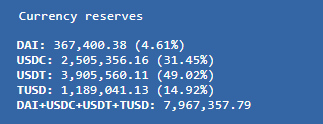
you would then get 46.1 DAI, 314.5 USDC, 490.2 USDT and 149.2 TUSD. Those values change constantly as people trade and arb. When you deposit, you will get a deposit bonus if the token you deposit has the lowest share. This tries to balance the pool to 25%, 25%, 25%, 25% by encouraging deposits of the rare stablecoin. Equally, widthdrawals can have a bonus if the chosen token has a high share.

Interest¶

To make the splitting of tokens and deposits more attractive,

the liquidity pools are also supplied to lending protocols like Compound (for cPool) in the background so you get extra interests on top of the trading fees.

The y pools (all the pools using yTokens: PAX, Y and BUSD) use a protocol called iEarn (which automatically rebalances the interest yield between Compound, Aave and dYdX).

Incentivised Pools¶

Staking REN (inter-blockchain token) and SNX (synthetix) in curve pools also results in additional interest from the token issuers.

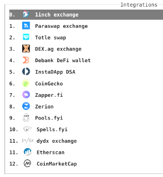
Current Integrations¶

(as of Oct. 8th, 2020) Current Integrations

Regulation¶

in Switzerland, if a DEX doesn’t have an ability to interfere with trades or stop them, KYC may not be needed (The devil is in the details, of course). However, that is why Curve is built without upgradeability and will be coordinated by a DAO.